|
|
||
|---|---|---|
| ml_models | ||
| notebooks | ||
| readme_data | ||
| scripts | ||
| .gitignore | ||
| LICENSE.txt | ||
| README.md | ||
| features.db | ||
| filter_params.json | ||
| requirements.txt | ||
| settings.json | ||
README.md
HSMA Data Science and Analytics SS2024
This project was developed through the Data Science and Analytics course at the Mannheim University of Applied Sciences. A data science cycle was taught theoretically on the basis of lectures and implemented practically in the project.
Analysis of cardiovascular diseases using ECG data
Table of Contents
About
Cardiovascular diseases refer to a group of diseases that affect the heart and blood vessels and represent a significant global health burden. They are a leading cause of morbidity and mortality worldwide, making effective prevention and management of these diseases critical. Physical examinations, blood tests, ECGs, stress or exercise tests, echocardiograms and CT or MRI scans are used to diagnose cardiovascular disease. (source: https://www.netdoktor.de/krankheiten/herzkrankheiten/, last visit: 15.05.2024)
An electrocardiogram (ECG) is a method of recording the electrical activity of the heart over a certain period of time. As an important diagnostic technique in cardiology, it is used to detect cardiac arrhythmias, heart attacks and other cardiovascular diseases. The ECG displays this electrical activity as waves and lines on a paper or screen. According to current screening and diagnostic practices, either cardiologists or physicians review the ECG data, determine the correct diagnosis and begin implementing subsequent treatment plans such as medication regimens and radiofrequency catheter ablation. (https://flexikon.doccheck.com/de/Elektrokardiogramm, last visit: 15.05.2024)
The project uses a dataset from a 12-lead electrocardiogram database published in August 2022. The database was developed under the auspices of Chapman University, Shaoxing People's Hospital and Ningbo First Hospital to support research on arrhythmias and other cardiovascular diseases. The dataset contains detailed data from 45,152 patients, recorded at a sampling rate of 500 Hz, and includes several common rhythms as well as additional cardiovascular conditions. The diagnoses are divided into four main categories: SB (sinus bradycardia), AFIB (atrial fibrillation and atrial flutter), GSVT (supraventricular tachycardia) and SR (sinus rhythm and sinus irregularities). The ECG data was stored in the GE MUSE ECG system and exported to XML files. A conversion tool was developed to convert the data to CSV format, which was later converted to WFDB format. (source: https://doi.org/10.13026/wgex-er52, last visit: 15.05.2024)
The data set used in this project was divided into four main groups: SB, AFIB, GSVT and SR. The choice of these groups is based on the results from the paper “Optimal Multi-Stage Arrhythmia Classification Approach” by Jianwei Zheng, Huimin Chu et al., this choice in turn is based on expert opinions from 11 physicians. Each group represents different cardiac arrhythmias that can be identified by electrocardiographic (ECG) features. (source: https://rdcu.be/dH2jI, last visit: 15.05.2024)
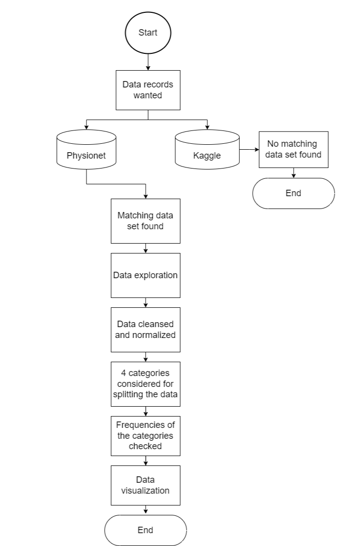
The data provision provides for the following points, which can be taken from the diagram.
Getting Started
This project is implemented in Python. Follow these steps to set up and use the project:
Prerequisites
- Ensure you have Python 3.8 or newer installed on your system.
- At least
10 GBof available disk space and32 GBof RAM are recommended for optimal performance.
Installation
-
Download the Dataset:
- Visit the dataset page (last visited: 15.05.2024) and download the dataset.
- Extract the dataset to a known directory on your system.
-
Install Dependencies:
- Open a terminal and navigate to the project directory.
- Run
pip install -r requirements.txtto install the required Python packages.
-
Configure the Project:
- Open the
settings.jsonfile in the project directory. - Adjust the parameters as needed, especially the path variables to match where you extracted the dataset.
- Open the
Generating Data
-
Generate Basic Data Files:
- In the terminal, ensure you are in the project directory.
- Run
generate_data.pymain-functionwith the folloing parametersgen_data=Truegen_features=Falseto generate several pickle files. This process may take some time.
-
Generate Machine Learning Features (Optional):
- Run
generate_data.pymain-functionwith the folloing parametersgen_data=Falsegen_features=Trueto generate a databse file.dbfor machine learning features. This also may take some time.
- Run
Using the Project
- With the data generated, you can now proceed to use the notebooks and other data as intended in the project.
Please refer to the individual notebook files for specific instructions on running analyses or models.
Usage
Let's walk through a user story to illustrate how to use our project, incorporating the updated "Getting Started" instructions:
User Story: Analyzing Health Data with Emma
Emma, a health data analyst, is keen on exploring the relationship between ECG Signals and health outcomes. She decides to use our project for her analysis. Here's how she proceeds:
-
Preparation:
- Emma checks that her computer has at least 10GB of free space and 32GB of RAM.
- She visits the dataset page (https://doi.org/10.13026/wgex-er52, last visited: 15.05.2024) and downloads the dataset.
- After downloading, Emma extracts the data to a specific directory on her computer.
-
Setting Up:
- Emma opens a terminal, navigates to the project directory, and runs
pip install -r requirements.txtto install the required Python packages. - She opens the
settings.jsonfile in the project directory and adjusts the parameters, especially the path variables to match the directory where she extracted the dataset.
- Emma opens a terminal, navigates to the project directory, and runs
-
Generating Data:
- To generate basic data files, Emma ensures she's in the project directory in the terminal. She then runs
generate_data.pyand manually adjusts the script beforehand to call themainfunction withgen_data=Trueandgen_features=False. This process generates several pickle files and may take some time. - For generating machine learning features (optional), Emma adjusts the script to call the
mainfunction withgen_data=Falseandgen_features=Trueto generate a database file.db. This also may take some time.
- To generate basic data files, Emma ensures she's in the project directory in the terminal. She then runs
-
Analysis:
- With the data and features generated, Emma is now ready to dive into the analysis. She opens the provided Jupyter notebooks and can see the demographic plots, methods of feature detection and noise reduction. With the
filter_params.jsonfile she is also able to adujst paramters to see how it changes the noise reducing.
- With the data and features generated, Emma is now ready to dive into the analysis. She opens the provided Jupyter notebooks and can see the demographic plots, methods of feature detection and noise reduction. With the
-
Deep Dive:
- Interested in the features and the resulting machine learning accurarcies, Emma uses the signal processing notebooks to analyze patterns in the health data.
- She adjusts parameters and runs different analyses, noting interesting trends and correlations.
- After Training her own models, she can also compare here results with the included models of the
ml_modelsdirectionary to evaluate the performance of her models.
-
Sharing Insights:
- Emma compiles her findings into a report, using plots and insights generated from our project.
- She shares her report with her team, highlighting how features like the R Axis can influence health outcomes.
Through this process, Emma was able to leverage our project to generate meaningful insights into health data, demonstrating the project's utility in real-world analysis.
Progress
- Data was searched and found at : (https://doi.org/10.13026/wgex-er52, last visit: 15.05.2024)
- Data was cleaned
- Demographic data was plotted
- Hypotheses put forward
- Start exploring signal processing
Data cleaning
The following criteria were checked to ensure data quality:
- Number of data records that did not specify gender
- Number of data sets that did not specify an age
- Number of data records in which the signal length deviates from 5000 (10 seconds * 500 Hz)
- Number of data records that could not be read in
Demographic plots
Histogram
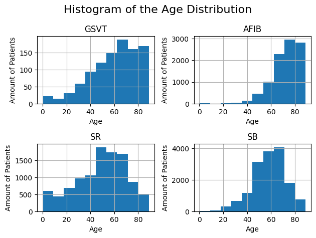
The following histogram shows the age distribution. It illustrates the breakdown of the grouped diagnoses by age group as well as the absolute frequencies of the diagnoses.
The exact procedure for creating the histogram can be found in the notebook demographic_plots.ipynb.
Correlation matrix
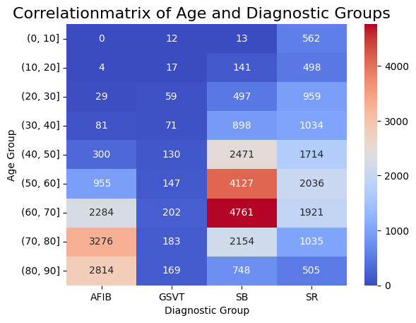
The following figure shows a correlation matrix of age groups and diagnoses. This matrix describes the four diagnosis groupings on the horizontal axis and the age groupings in decade increments on the vertical axis.
The colour scale represents the correlation between the two types of categorization:
- Blue (low)
- Red (high)
The exact procedure for creating the matrix can be found in the notebook demographic_plots.ipynb.
Hypotheses
The following two hypotheses were applied in this project:
Hypotheses 1:
-
Using ECG data, a classifier can classify the four diagnostic groupings with an accuracy of at least 80%.
Result:
- For the first hypothesis, an accuracy of 83 % was achieved with the XGBoost classifier. The detailed procedure can be found in the following notebook: ml_xgboost.ipynb
- Also a 82 % accuracy was achieved with a Gradient Boosting Tree Classifier. The detailed procedure can be found in the following notebook: ml_grad_boost_tree.ipynb
With those Classifiers, the hypothesis can be proven, that a classifier is able to classify the diagnostic Groups with a accuracy of at least 80%.
Hypotheses 2:
-
Sinus bradycardia occurs significantly more frequently in the 60 to 70 age group than in other age groups.
The second hypothesis was tested for significance using the chi-square test. The detailed procedure can be found in the following notebook: statistics.ipynb
Result:
-
The first value returned is the Chi-Square Statistic that shows the difference between the observed and the expected frequencies. Here, a bigger number indicates a bigger difference. The p-value shows the probability of this difference being statistically significant. If the p-value is below the significance level of 0.05, the difference is significant.
-
The Chi-Square Statistic for sinus bradycardia in the age group 60-70 compared to the other age groups, is a value that shows whether there is a significant difference in the frequency of sinus bradycardia in the age group 60-70 in comparison to the other age groups. If the p-value is smaller than the significance level of 0.05, the difference in the frequency between the age group 60-70 and the other age groups is significant.
The significant appearance of sinus bradycardia in the age group 60-70 could be caused by multiple factors. In this case the physiological age could play a huge factor. The sinus node continuously generates electrical impulses, thus setting the normal rhythm and rate in a healthy heart. With increasing age, the sinus node becomes less responsive which leads to a slower heart rate of 60 bpm or less. Another reason could be increased medication, which is more likely to be the case when older. A sinus bradycardia could appear as a side effect of that medication.
(source: https://doi.org/10.1253/jcj.57.760, last visit: 10.06.2024)
(source: https://doi.org/10.7861%2Fclinmed.2022-0431, last visit: 10.06.2024)But what could be the reason for the more frequent appearance of the sinus bradycardia in the age group 60-70 than in other older age groups?
The lower number of sinus bradycardia cases in older age groups could be due to the increasing mortality with higher ages. People with sinus bradycardia might not reach older ages because of comorbidities and further complications. Besides that, older people are more likely to receive medical support such as medication and pacemakers which can prevent sinus bradycardia or at least lower its effect. The sample size in the study conducted may also play a role in the significance of the frequency.
Contributing
Thank you for your interest in contributing to our project! As an open-source project, we welcome contributions from everyone. Here are some ways you can contribute:
-
Reporting Bugs: If you find a bug, please open an issue on our GitHub page with a detailed description of the bug, steps to reproduce it, and any other relevant information that could help us fix it.
-
Suggesting Enhancements: Have ideas on how to make this project better? Open an issue on our GitHub page with your suggestions.
-
Pull Requests: Ready to contribute code or documentation? Great! Please follow these steps:
- Fork the repository.
- Create a new branch for your feature or fix.
- Commit your changes with clear, descriptive commit messages.
- Push your changes to your branch.
- Submit a pull request to our repository. Include a clear description of your changes and the purpose of them.
Please note, by contributing to this project, you agree that your contributions will be licensed under its MIT License.
We look forward to your contributions. Thank you for helping us improve this project!
License
This project is licensed under the MIT License.
Acknowledgements
We would like to especially thank our instructor, Ms. Jacqueline Franßen, for her enthusiastic support in helping us realize this project.
Contact
- Klara Tabea Bracke (3015256@hs-mannheim.de)
- Arman Ulusoy (3016148@stud.hs-mannheim.de)
- Nils Rekus (1826514@stud.hs-mannheim.de)
- Felix Jan Michael Mucha (felixjanmichael.mucha@stud.hs-mannheim.de)


