DSA_SS24/README.md

HSMA Data Science and Analytics SS2024

This project was developed as part of the Data Science and Analytics course at the Mannheim University of Applied Sciences. A data science cycle was taught theoretically in lectures and implemented practically in the project.

Analysis of cardiovascular diseases using ECG data

Table of Contents

• About
• Getting Started
• Usage
• Progress
• Contributing
• License
• Acknowledgements
• Contact

About

(as of 12.06)

Cardiovascular diseases are a group of diseases that affect the heart and blood vessels and represent a significant global health burden. They are a leading cause of morbidity and mortality worldwide, making effective prevention and management of these diseases critical. Physical examinations, blood tests, ECGs, stress or exercise tests, echocardiograms and CT or MRI scans are used to diagnose cardiovascular disease. (source: https://www.netdoktor.de/krankheiten/herzkrankheiten/, last visit: 15.05.2024)

An electrocardiogram (ECG) is a method of recording the electrical activity of the heart over a certain period of time. As an important diagnostic technique in cardiology, it is used to detect cardiac arrhythmias, heart attacks and other cardiovascular diseases. The ECG displays this electrical activity as waves and lines on paper or on a screen. According to current screening and diagnostic practices, either cardiologists or physicians review the ECG data, determine the correct diagnosis and begin implementing subsequent treatment plans such as medication regimens and radiofrequency catheter ablation. (https://flexikon.doccheck.com/de/Elektrokardiogramm, last visit: 15.05.2024)

The project uses a dataset from a 12-lead electrocardiogram database published in August 2022. The database was developed under the auspices of Chapman University, Shaoxing People's Hospital and Ningbo First Hospital to support research on arrhythmias and other cardiovascular diseases. The dataset contains detailed data from 45,152 patients, recorded at a sampling rate of 500 Hz, and includes several common rhythms as well as additional cardiovascular conditions. The diagnoses are grouped into four main categories: SB (sinus bradycardia), AFIB (atrial fibrillation and atrial flutter), GSVT (supraventricular tachycardia) and SR (sinus rhythm and sinus irregularities). The ECG data was stored in the GE MUSE ECG system and exported to XML files. A conversion tool was developed to convert the data to CSV format, which was later converted to WFDB format. (source: https://doi.org/10.13026/wgex-er52, last visit: 15.05.2024)

The dataset used in this project was divided into four main groups: SB, AFIB, GSVT and SR. The choice of these groups is based on the results from the paper “Optimal Multi-Stage Arrhythmia Classification Approach” by Jianwei Zheng, Huimin Chu et al., this choice in turn is based on expert opinions from 11 physicians. Each group represents different cardiac arrhythmias that can be identified by electrocardiographic (ECG) features. (source: https://rdcu.be/dH2jI, last visit: 15.05.2024)

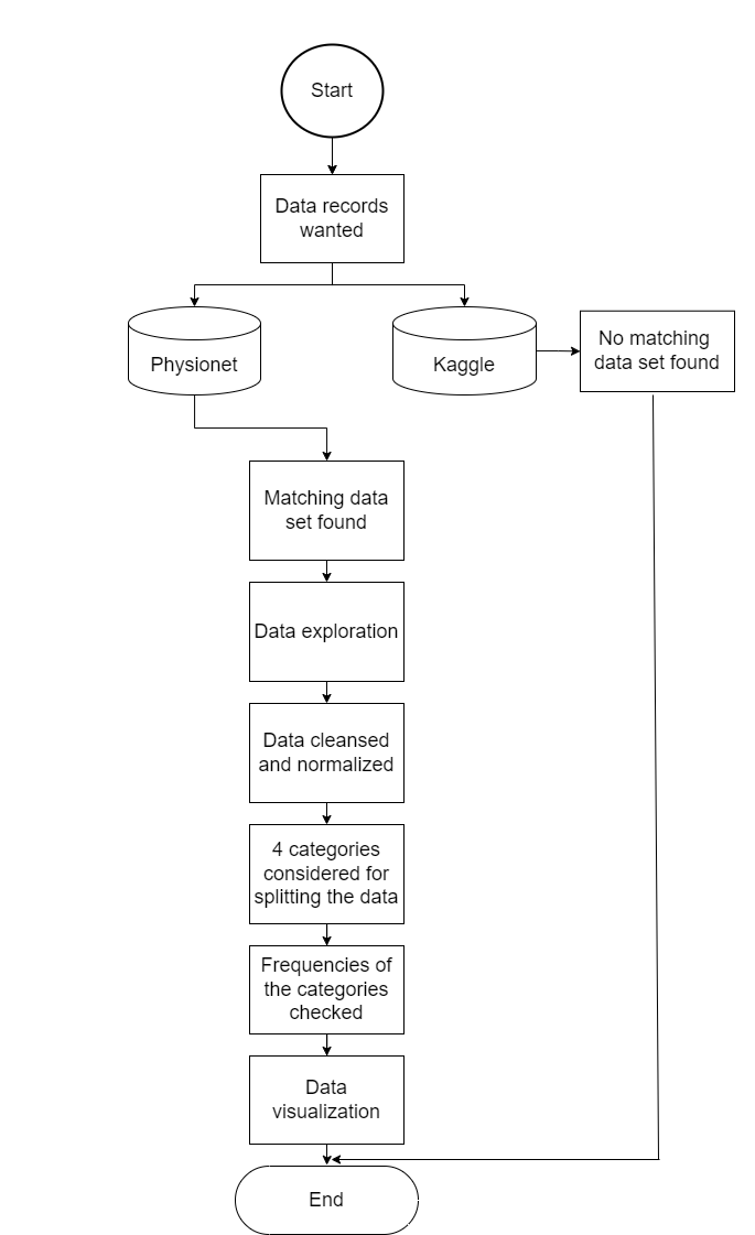
The data provision provides for the following points, which can be taken from the diagram.

Getting Started

(as of 12.06) This project is implemented in Python. Follow these steps to set up and use the project:

Prerequisites

(as of 12.06)

• Ensure you have Python 3.8 or newer installed on your system.
• At least 10 GB of available disk space and 32 GB of RAM are recommended for optimal performance.

Installation

(as of 12.06)

1. Download the Dataset:

   • Visit the dataset page (last visited: 15.05.2024) and download the dataset.
   • Extract the dataset to a known directory on your system.

2. Install Dependencies:

   • Open a terminal and navigate to the project directory.
   • Run pip install -r requirements.txt to install the required Python packages.

3. Configure the Project:

   • Open the settings.json file in the project directory.
   • Adjust the parameters as needed, especially the path variables to match where you extracted the dataset.

Generating Data

(as of 12.06)

1. Generate Basic Data Files:

   • In the terminal, ensure you are in the project directory.
   • Run generate_data.py main-function with the folloing parameters gen_data=True gen_features=False to generate several pickle files. This process may take some time.

2. Generate Machine Learning Features (Optional):

   • Run generate_data.py main-function with the folloing parameters gen_data=False gen_features=True to generate a databse file .db for machine learning features. This also may take some time.

Using the Project

• With the data generated, you can now proceed to use the notebooks and other data as intended in the project.

Please refer to the individual notebook files for specific instructions on running analyses or models.

Usage

Let's walk through a user story to illustrate how to use our project, incorporating the updated "Getting Started" instructions:

User Story: Analyzing Health Data with Emma

Emma, a health data analyst, is keen on exploring the relationship between ECG Signals and health outcomes. She decides to use our project for her analysis. Here's how she proceeds:

1. Preparation:

   • Emma makes sure that her computer has at least 10GB of free space and 32GB of RAM.
   • She visits the dataset page (https://doi.org/10.13026/wgex-er52, last visited: 15.05.2024) and downloads the dataset.
   • After the download, Emma extracts the data to a specific directory on her computer.

2. Setting Up:

   • Emma opens a terminal, navigates to the project directory, and runs pip install -r requirements.txt to install the required Python packages.
   • She opens the settings.json file in the project directory and adjusts the parameters, especially the path variables to match the directory where she extracted the dataset.

3. Generating Data:

   • To generate basic data files, Emma ensures she's in the project directory in the terminal. She then runs generate_data.py and manually adjusts the script beforehand to call the main function with gen_data=True and gen_features=False. This process generates several pickle files and may take some time.
   • For generating machine learning features (optional), Emma adjusts the script to call the main function with gen_data=False and gen_features=True to generate a database file .db. This may also take some time.

4. Analysis:

   • With the data and features generated, Emma is now ready to dive into the analysis. She opens the provided Jupyter notebooks and can see the demographic plots, methods of feature detection and noise reduction. With the filter_params.json file she is also able to adjust paramters to see how it changes the noise reduction.

5. Deep Dive:

   • Interested in the features and the resulting machine learning accuracies, Emma uses the signal processing notebooks to analyze patterns in the health data.
   • She adjusts parameters and runs different analyses, noting interesting trends and correlations.
   • After Training her own models, she can also compare here results with the included models of the ml_models directionary to evaluate the performance of her models.

6. Sharing Insights:

   • Emma compiles her findings into a report, using plots and insights generated from our project.
   • She shares her report with her team, highlighting how features like the R axis can influence health outcomes.

Through this process, Emma was able to leverage our project to generate meaningful insights into health data, demonstrating the project's utility in real-world analysis.

Progress

• Data was searched and found at : (https://doi.org/10.13026/wgex-er52, last visit: 15.05.2024)
• Data was cleaned (as of 12.06)
• Demographic data was plotted (as of 12.06)
• Hypotheses put forward (as of 12.06 & 03.07)
• Noise reduction (as of 12.06)
• Features(as of 12.06)
• ML-models (as of 12.06 & 03.07)
• Cluster analysis (as of 03.07)
• Legal basis (as of 03.07)
• Conclusion (as of 03.07)
• Outlook (as of 03.07)

Data cleaning

(as of 12.06)

The following criteria were checked to ensure data quality:

• Number of data records that did not specify gender
• Number of datasets that did not specify an age
• Number of data records in which the signal length deviates from 5000 (10 seconds * 500 Hz)
• Number of data records that could not be read in

Demographic plots

(as of 12.06)

Histogram

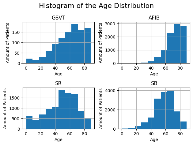
The following histogram shows the age distribution. It illustrates the breakdown of the grouped diagnoses by age group as well as the absolute frequencies of the diagnoses.

The exact procedure for creating the histogram can be found in the notebook demographic_plots.ipynb.

Correlation matrix

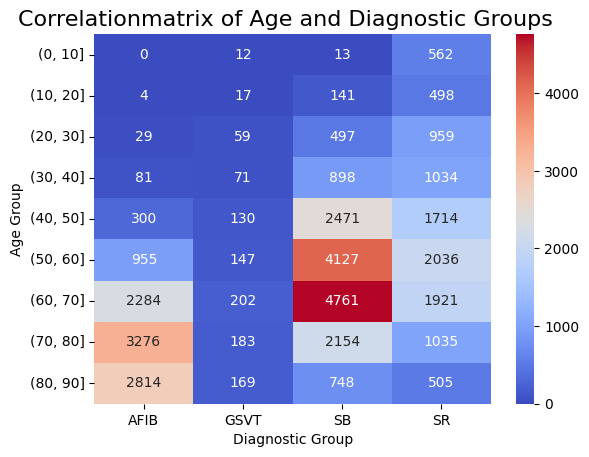
The following figure shows a correlation matrix of age groups and diagnoses. This matrix describes the four diagnosis groupings on the horizontal axis and the age groupings in decade increments on the vertical axis.

The colour scale represents the correlation between the two types of categorization:

• Blue (low)
• Red (high)

Notably, the age group between 60-70 in SB shows a noticeably higher correlation and will therefore be considered in our hypothesis analysis. The other groups align mostly as expected, with a slight increase in correlation observed with age.

The exact procedure for creating the matrix can be found in the notebook demographic_plots.ipynb.

Hypotheses

(as of 03.07.)

The following two hypotheses were applied in this project:

Hypotheses 1:

1. Using ECG data, a classifier can classify the four diagnostic groupings with an accuracy of at least 80%.

   Result:

• For the first hypothesis, an accuracy of 83 % was achieved with the XGBoost classifier. The detailed procedure can be found in the following notebook: ml_xgboost.ipynb (as of 12.06)
• Also a 82 % accuracy was achieved with a Gradient Boosting Tree Classifier. The detailed procedure can be found in the following notebook: ml_grad_boost_tree.ipynb (as of 12.06)
• An 80 % accuracy was achieved with a Decision Tree Classifier. The detailed procedure can be found in the following notebook: ml_decision_tree.ipynb (as of 03.07)

With those Classifiers, the hypothesis can be proven, that a classifier is able to classify the diagnostic Groups with a accuracy of at least 80%.

Hypothesis 2:

2. Sinus bradycardia occurs significantly more frequently in the 60 to 70 age group than in other age groups. Atrial fibrillation/atrial flutter also occurs significantly more frequently in the 70 to 80 age group than in other age groups.
   The second hypothesis was tested for significance using the Chi-square test. The detailed procedure can be found in the following notebook: statistics.ipynb

   Results:

• The first value returned for both tests is the Chi-Square Statistic (1043.5644539016944) that shows the difference between the observed and the expected frequencies. Here, a bigger number indicates a bigger difference. The p-value shows the probability of this difference being statistically significant. The p-value (4.935370162055676e-205) is below the significance level of 0.05, meaning the difference is significant.

• The Chi-Square Statistic (32.94855579340837) for sinus bradycardia in the age group 60-70 compared to the other age groups, is a value that shows whether there is a significant difference in the frequency of sinus bradycardia in the age group 60-70 in comparison to the other age groups. If the p-value (9.463001659861763e-09) is smaller than the significance level of 0.05, the difference in the frequency between the age group 60-70 and the other age groups is significant.
  The same approach is taken for atrial fibrillation/atrial flutter in the age group of 70-80 compared to the other age groups. the Chi-Square Statistic (120.60329273774582) shows the significant difference in the frequency of atrial fibrillation/atrial flutter in the age group 70-80 in comparison to the other age groups. The p-value (4.667227334873944e-28) is smaller than the significance level of 0.05, therefore the difference in the frequency between the age group 70-80 and the other age groups is significant.

The significant appearance of sinus bradycardia in the age group 60-70 could be caused by multiple factors. In this case, the physiological age could play a huge factor. The sinus node continuously generates electrical impulses, thus setting the normal rhythm and rate in a healthy heart. With increasing age, the sinus node becomes less responsive which leads to a slower heart rate of 60 bpm or less. Another reason could be increased medication, which is more likely to be the case when older. A sinus bradycardia could appear as a side effect of that medication.
(source: https://doi.org/10.1253/jcj.57.760, last visit: 10.06.2024)
(source: https://doi.org/10.7861%2Fclinmed.2022-0431, last visit: 10.06.2024)

But what could be the reason for the more frequent appearance of the sinus bradycardia in the age group 60-70 than in other older age groups?

The lower number of sinus bradycardia cases in older age groups could be due to the increasing mortality with higher ages. People with sinus bradycardia might not reach older ages because of comorbidities and further complications. Besides that, older people are more likely to receive medical support such as medication and pacemakers which can prevent sinus bradycardia or at least lower its effect. The higher frequency of older people in the database may lead to a slight bias in the distribution. See also Demographic Bias.
The sample size in the study conducted may also play a role in the significance of the frequency.

The significant appearance of atrial fibrillation/atrial flutter in the age group 70-80 could be caused by multiple factors. The physiological age is the main reason. With increasing age, various age-related changes in the cardiovascular system occur. Older people are more likely to have hypertension. The increased pressure can lead to thickening of the heart walls and a change of the structure, potentially leading to AFIB. Chronic inflammation which is more prevalent in older people, can damage heart tissue and lead to atrial issues. The change of hormone levels when getting older can also have an influence on the heart function and contribute to the development of arrhythmias. Older adults are also more likely to have comorbidities such as diabetes, obesity or chronic kidney disease.
(source: https://www.ncbi.nlm.nih.gov/pmc/articles/PMC5460064/, last visit: 28.06.2024)

Noise reduction

(as of 12.06)

Noise suppression was performed on the existing ECG data. A three-stage noise reduction was performed to reduce the noise in the ECG signals. First, a Butterworth filter was applied to the signals to remove the high frequency noise. Then a Loess filter was applied to the signals to remove the low frequency noise. Finally, a non-local-means filter was applied to the signals to remove the remaining noise. For noise reduction, the built-in noise reduction function from NeuroKit2 ecg_clean was utilized for all data due to considerations of time performance.

How the noise reduction was performed in detail can be seen in the following notebook: noise_reduction.ipynb

Features

(as of 12.06) The detection ability of the NeuroKit2 library is tested to detect features in the ECG dataset. Those features are important for the training of the model in order to detect the different diagnostic groups. The features are detected using the NeuroKit2 library.

For the training, the features considered are:

• ventricular rate
• atrial rate
• T axis
• R axis
• Q peak amplitude
• QT length
• QRS duration
• QRS count
• gender
• age

The selection of features was informed by an analysis presented in a paper (source: https://rdcu.be/dH2jI, last accessed: 15.05.2024), where various feature sets were evaluated. These features were chosen for their optimal balance between performance and significance.

The exact process can be found in the notebook: features_detection.ipynb.

ML-models

For machine learning, the initial step involved tailoring the features for the models, followed by employing a grid search to identify the best hyperparameters. This approach led to the highest performance being achieved by the Extreme Gradient Boosting (XGBoost) model, which attained an accuracy of 83%. Additionally, a Gradient Boosting Tree model was evaluated using the same procedure and achieved an accuracy of 82%. A Decision Tree model was also evaluated, having the lowest performance of 80%. The selection of these models was influenced by the team's own experience and the performance metrics highlighted in the paper (source: https://rdcu.be/dH2jI, last accessed: 15.05.2024). The models have also been evaluated, and it is noticeable that some features, like the ventricular rate, are shown to be more important than other features.

The detailed procedures can be found in the following notebooks:
ml_xgboost.ipynb(as of 12.06)
ml_grad_boost_tree.ipynb (as of 12.06)
ml_decision_tree.ipynb (as of 03.07)

Cluster-analysis

(as of 03.07)

To enhance our understanding of the feature clusters and their similarity to the original data labels, we began our analysis by preparing the data. This preparation included normalization and imputation of missing values with mean substitution. Subsequently, we employed the K-Means algorithm for distance-based clustering of the data. Our exploration focused on comparing two types of labels: those derived from the K-Means algorithm and the original dataset labels. Various visualizations were generated to facilitate this comparison.

A dimensionality reduction plot using Principal Component Analysis (PCA) revealed that, although the clusters formed by the K-Means algorithm and the original labels are not highly similar, both exhibit some degree of clustering. To quantitatively assess the quality of the K-Means clusters, we calculated the following metrics:

• Adjusted Rand Index (ARI): 0.15
• Normalized Mutual Information (NMI): 0.24
• Silhouette Score: 0.47

The ARI and NMI scores indicate that the clustering algorithm has a moderate level of effectiveness in reflecting the structure of the true labels, although not with high accuracy. These scores suggest some alignment with the true labels, but the clustering does not perfectly capture the underlying groupings. This suggests that the distances between features, as determined by the clustering algorithm, do not fully reflect the inherent categorizations indicated by the original labels of the data.

The Silhouette Score suggests that the clusters identified are internally coherent and distinct from each other, indicating that the clustering algorithm has been somewhat successful in identifying meaningful structures within the data, even if these structures do not align perfectly with the true labels.

Further analysis included the creation of a Euclidean distance matrix plot to visualize patterns of data point separation. This analysis revealed the presence of outliers, as some data points were significantly more distant from others.

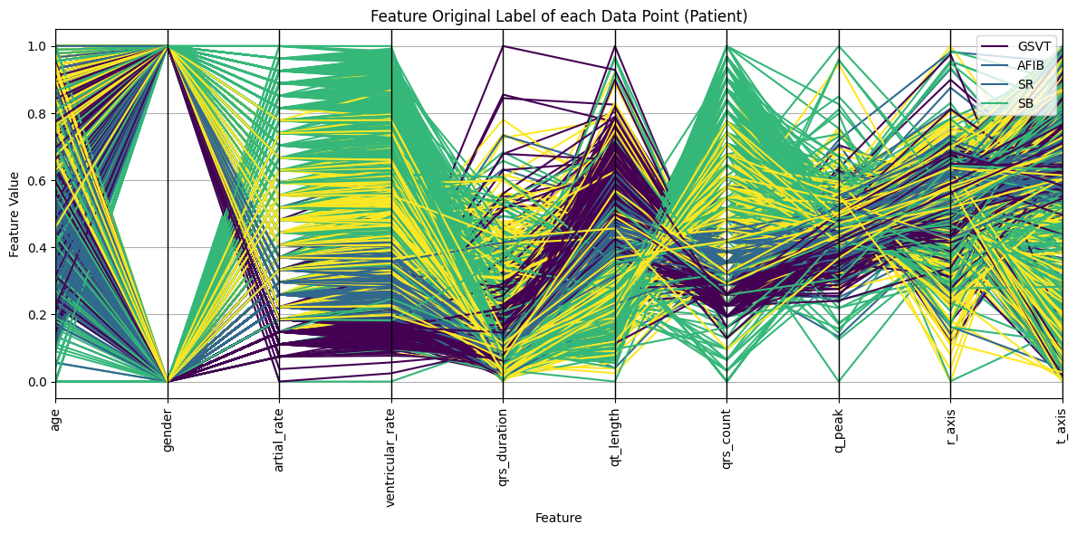
Finally, a parallel axis plot was generated to examine the relationship between the data features and the clusters. Notably, this plot highlighted the ventricular rate feature as a significant separator in the original labels, underscoring its importance as identified by our machine learning models in predicting the labels.

The detailed procedures can be found in the following notebook:
cluster_features.ipynb

Data Biases

(as of 03.07)

Local Bias

• The dataset originates exclusively from one hospital, including contributions from Chapman University, Shaoxing People’s Hospital (affiliated with Shaoxing Hospital Zhejiang University School of Medicine), and Ningbo First Hospital. This may introduce a local bias, as all data are collected from a specific geographic and institutional context.

Demographic Bias

• The dataset predominantly features data from older individuals, with the majority of participants falling within the 60-70 age group. This demographic skew is further detailed by:
  • Average age: 59.59 years
  • Standard deviation of age: 18.29 years
  • Male ratio: 57.34%
  • Female ratio: 42.66% This indicates a potential demographic bias towards older age groups and a gender imbalance.

Data protection and ethics

(as of 03.07)

The data used in the project was approved by the review boards of Shaoxing People's Hospital and Ningbo First Hospital of Zhejiang University. Both institutions allowed public disclosure of the data after de-identification. While Shaoxing People's Hospital additionally waived the informed consent requirement, Ningbo First Hospital also did not require patient consent.

Conclusion

(as of 03.07)

This project has impressively demonstrated the feasibility and benefits of applying modern data analysis methods and machine learning in the field of cardiology. By using a large dataset of 12-lead ECGs, it was possible to effectively classify different cardiac arrhythmias using models such as XGBoost, gradient boosting and decision trees. These models achieved classification accuracies of and above 80%, highlighting the importance of accurate diagnostic tools.

Despite these successes, we encountered challenges such as the lack of datasets for certain demographic groups and the handling of incomplete ECG recordings. These limitations highlight the need for further research to improve data collection and processing in medical studies.

The application of these analytical techniques not only provides the opportunity for more accurate and faster diagnoses, but also opens avenues for the development of personalized treatment approaches tailored to specific patient-individual data.

Ultimately, our research shows that the continued integration and improvement of technological solutions in medical diagnostic procedures is essential for future healthcare. We recommend continuing research in this direction.

Outlook

(as of 03.07)

As data science advances, there are several opportunities to improve and extend current research on cardiovascular disease analysis using ECG data.
Key future directions include:

• Advanced machine learning techniques: Incorporating more machine learning methods such as deep learning could improve the accuracy and reliability of cardiovascular disease diagnosis.

• Expansion of features used: Future developments could include expanding the feature sets used. By adding new predictive features or enhancing existing features, the precision of the models could be further improved.

• Data augmentation: Data augmentation techniques could be used to solve problems such as unbalanced datasets or underrepresented classes. This would help to create a more robust model by generating synthetic ECG data that provides the machine learning models with more examples to learn from.

• Integration of additional data sources: Expanding the database to include more diverse datasets from different geographic and demographic contexts could help mitigate local and demographic biases.

• Visual data comparsion: With the use of the given ECG data there could be calculated a "standardized" QRS-Complex for every diagnosis group examined in this program, to classify new unknown ECG data with no prior diagnosis.

Contributing

(as of 12.06)

Thank you for your interest in contributing to our project! As an open-source project, we welcome contributions from everyone. Here are some ways you can contribute:

• Reporting Bugs: If you find a bug, please open an issue on our GitHub page with a detailed description of the bug, steps to reproduce it, and any other relevant information that could help us fix it.

• Suggesting Enhancements: Have ideas on how to make this project better? Open an issue on our GitHub page with your suggestions.

• Pull Requests: Ready to contribute code or documentation? Great! Please follow these steps:

  1. Fork the repository.
  2. Create a new branch for your feature or fix.
  3. Commit your changes with clear, descriptive commit messages.
  4. Push your changes to your branch.
  5. Submit a pull request to our repository. Include a clear description of your changes and the purpose of them.

Please note that by contributing to this project, you agree that your contributions will be licensed under its MIT License.

We look forward to your contributions. Thank you for helping us improve this project!

License

This project is licensed under the MIT License.

Acknowledgements

We would like to especially thank our instructor, Ms. Jacqueline Franßen, for her enthusiastic support in helping us realize this project.

Contact

• Klara Tabea Bracke (3015256@hs-mannheim.de)
• Arman Ulusoy (3016148@stud.hs-mannheim.de)
• Nils Rekus (1826514@stud.hs-mannheim.de)
• Felix Jan Michael Mucha (felixjanmichael.mucha@stud.hs-mannheim.de)